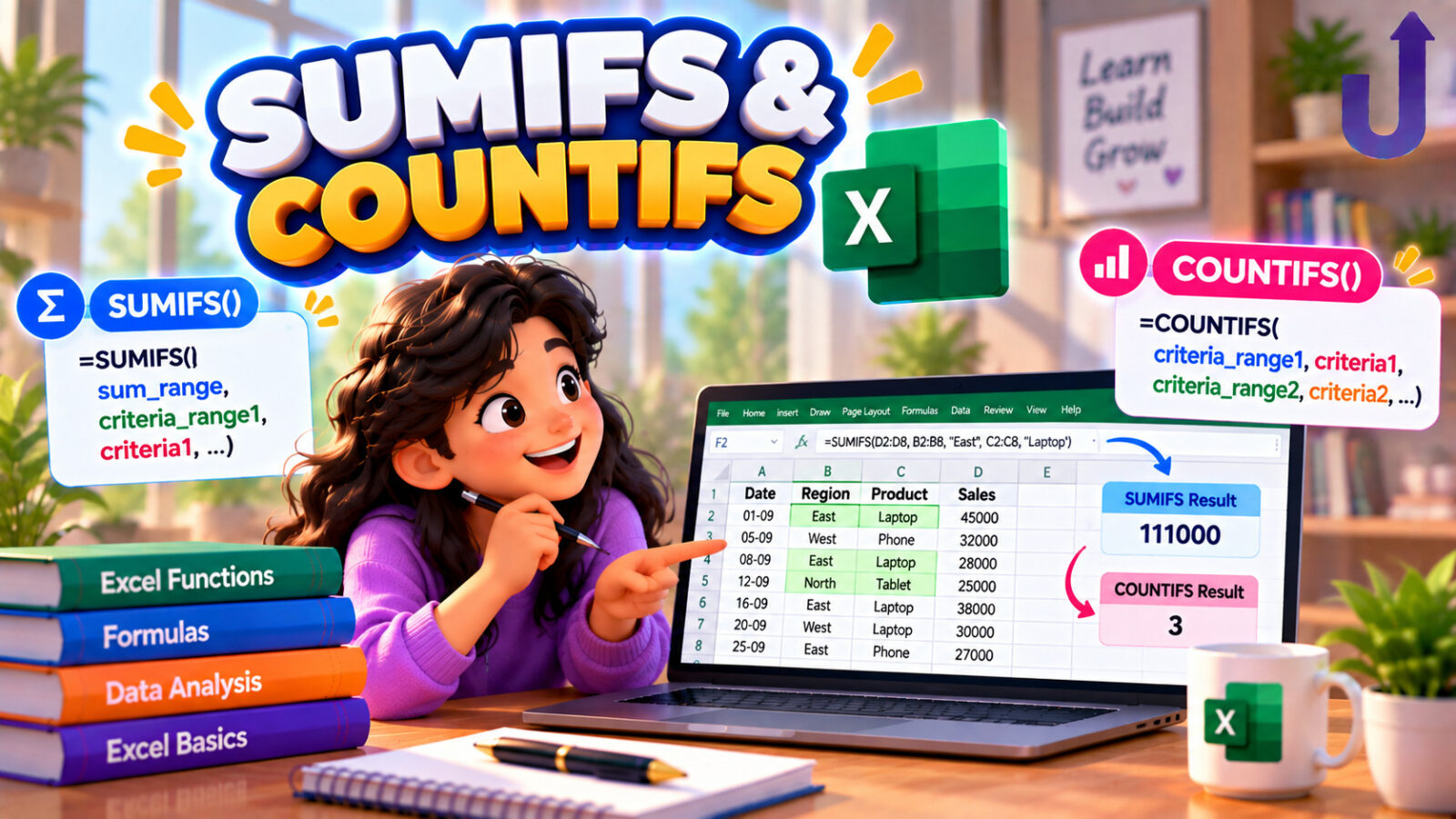
SUMIFS, COUNTIFS and AVERAGEIFS are the Excel functions that add, count and average only the rows that meet conditions you set. SUMIFS totals a column for the rows that match, COUNTIFS counts them, and AVERAGEIFS averages them. Each condition is a pair of a range and a criterion, for example B2:B11, "North", and when there are several pairs a row must satisfy all of them. Older single-condition versions, SUMIF, COUNTIF and AVERAGEIF, still work.
This guide uses one small sales table throughout, shows how to write criteria (text, numbers, wildcards, dates, cell references), how to handle OR conditions and the AND-with-OR combination that SUMIFS does not do directly, and the traps that give quietly wrong totals. Every result was produced by running the formula in Microsoft Excel.
In this guide
The short version
=SUMIFS(sum_range, criteria_range1, criteria1, criteria_range2, criteria2, ...). The sum range comes first, and every range must have the same size.- Several conditions are combined with AND. For OR, add two results or give an array constant, such as
{"North","East"}. - Criteria such as
">=500","<>North"and"B*"are text; to use a value from a cell, join it with&:">="&H2. SUMIFputs the sum range last. Mixing the two orders up is a classic mistake.
The sample data
All examples use this table of ten sales, in A1:E11. Amounts are in column D, so most formulas sum, count or average D2:D11:
| A | B | C | D | E | |
|---|---|---|---|---|---|
| 1 | Date | Region | Product | Amount | Paid |
| 2 | 2024-01-05 | North | Pen | 500 | Yes |
| 3 | 2024-01-18 | South | Book | 300 | No |
| 4 | 2024-02-02 | North | Book | 700 | Yes |
| 5 | 2024-02-14 | East | Pen | 200 | Yes |
| 6 | 2024-02-27 | South | Pen | 900 | No |
| 7 | 2024-03-03 | North | Bag | 400 | Yes |
| 8 | 2024-03-15 | East | Book | 600 | Yes |
| 9 | 2024-03-21 | South | Bag | 150 | No |
| 10 | 2024-03-30 | North | Pen | 350 | Yes |
| 11 | 2024-04-08 | East | Bag | 250 | No |
SUMIF and SUMIFS
SUMIF(range, criteria, [sum_range]) adds the cells of sum_range where range meets one condition. SUMIFS handles one or more conditions, and it turns the arguments around: the range to add comes first. Each extra condition is another pair of range and criteria:
| Formula | Excel shows | Why |
|---|---|---|
| =SUM(D2:D11) | 4350 | everything, for comparison |
| =SUMIF(B2:B11,"North",D2:D11) | 1950 | one condition: North (500 + 700 + 400 + 350) |
| =SUMIFS(D2:D11,B2:B11,"North",C2:C11,"Pen") | 850 | two conditions, both must hold: North Pens (500 + 350) |
| =SUMIFS(D2:D11,D2:D11,">=500") | 2700 | a range can be its own criteria range: sales of 500 or more |
| =SUMIFS(D2:D11,B2:B11,"<>North") | 2400 | every region except North |
| =SUMIFS(D2:D11,A2:A11,">="&DATE(2024,2,1),A2:A11,"<"&DATE(2024,3,1)) | 1800 | February only: from 1 February up to, not including, 1 March |
To filter dates, use two conditions on the same column, a start with >= and an end with < the first day of the next month. This also works when the dates contain times.
COUNTIFS, AVERAGEIFS, MAXIFS and MINIFS
The pattern is the same for counting and averaging. COUNTIFS takes only pairs of range and criteria, because there is nothing to add up. AVERAGEIFS takes the average range first, like SUMIFS. MAXIFS and MINIFS (Excel 2019 and Microsoft 365) find the biggest and smallest value among the matching rows:
| Formula | Excel shows | Why |
|---|---|---|
| =COUNTIFS(B2:B11,"South") | 3 | how many sales in the South |
| =COUNTIFS(B2:B11,"North",E2:E11,"Yes") | 4 | North and paid |
| =COUNTIFS(D2:D11,">=300",D2:D11,"<=600") | 5 | between 300 and 600 inclusive: two conditions on one column |
| =AVERAGEIFS(D2:D11,B2:B11,"East") | 350 | average of East's 200, 600 and 250 |
| =COUNTIFS(C2:C11,"B*") | 6 | products starting with B: Book and Bag |
| =COUNTIFS(E2:E11,"<>Yes") | 4 | everything that is not Yes |
| =MAXIFS(D2:D11,B2:B11,"South") | 900 | the biggest South sale |
| =MINIFS(D2:D11,B2:B11,"South") | 150 | the smallest South sale |
| =COUNTIF(B2:B11,"North")/COUNTA(B2:B11) | 0.4 | share of rows that are North |
Writing criteria
A criterion is a piece of text (or a number) that Excel interprets. These are the forms you will use:
| You want | Criterion | Example |
|---|---|---|
| Equal to a word | "North" (case does not matter) | =COUNTIFS(B2:B11,"north") counts the North rows |
| Not equal | "<>North" | everything except North |
| Greater or less than a number | ">=500", "<300" | the operator goes inside the quotes |
| Starts with, ends with, contains | "B*", "*k", "*oo*" | * stands for any run of characters |
| Exactly one unknown character | "?ast" | matches East; ? stands for one character |
| A real star or question mark | "~*", "~?" | the tilde switches the wildcard off |
| Blank cells | "" | or "<>" for cells that are not blank |
| A value held in a cell | ">="&H2 | join the operator to the cell with & |
| A date | ">="&DATE(2024,2,1) | never type a text date |
Putting the criteria in cells
Typing "East" inside the formula means you must edit the formula to change it. Put the criteria in cells and refer to them, and the same formula can be reused. Here H1 holds the region and H2 the minimum amount:
Criteria in H1 and H2, results in H4 to H6
| G | H | |
|---|---|---|
| 1 | Region | East |
| 2 | Minimum | 300 |
| 3 | ||
| 4 | 1050 | |
| 5 | 600 | |
| 6 | 1 |
What is inside the cells
| G | H | |
|---|---|---|
| 1 | Region | East |
| 2 | Minimum | 300 |
| 3 | ||
| 4 | =SUMIFS(D2:D11,B2:B11,H1) | |
| 5 | =SUMIFS(D2:D11,B2:B11,H1,D2:D11,”>”&H2) | |
| 6 | =COUNTIFS(B2:B11,H1,D2:D11,”>=”&H2) |
H4 adds all East sales (200 + 600 + 250). H5 adds only East sales above the minimum of 300, and H6 counts East sales of 300 or more. Note how the operator and the cell are joined: ">"&H2.
OR conditions
SUMIFS and COUNTIFS only know AND. There are three ways to get OR.
1. Add two results
North or East is the sum for North plus the sum for East. That is safe when a row cannot belong to both groups. A row cannot be in two regions at once.
2. Give an array constant
Write the alternatives in curly brackets and wrap the function in SUM: Excel runs the formula once per alternative and adds the results.
3. Combine AND with OR: where the brackets go
“North and (Pen or Bag)” keeps North as a fixed condition and lets the product vary. The array constant goes on the product only. The mirror rule, “(North and Pen) or Bag”, is a different question: it has to be two separate sums added together.
| Formula | Excel shows | Why |
|---|---|---|
| =SUMIFS(D2:D11,B2:B11,"North")+SUMIFS(D2:D11,B2:B11,"East") | 3000 | two SUMIFS added: North plus East |
| =SUM(SUMIFS(D2:D11,B2:B11,{"North","East"})) | 3000 | the array constant gives the same total in one formula |
| =SUM(SUMIFS(D2:D11,B2:B11,"North",C2:C11,{"Pen","Bag"})) | 1250 | North AND (Pen OR Bag): North Pens 850 + North Bags 400 |
| =SUMIFS(D2:D11,B2:B11,"North",C2:C11,"Pen")+SUMIFS(D2:D11,C2:C11,"Bag") | 1650 | (North AND Pen) OR Bag: 850 plus every Bag sale, 800 |
| =SUMIFS(D2:D11,B2:B11,"North")+SUMIFS(D2:D11,E2:E11,"Yes") | 4700 | WRONG for overlapping groups: rows that are North AND paid are added twice |
| =SUMIFS(D2:D11,B2:B11,"North")+SUMIFS(D2:D11,E2:E11,"Yes")-SUMIFS(D2:D11,B2:B11,"North",E2:E11,"Yes") | 2750 | correct union: add both, then subtract the overlap once |
| =SUMPRODUCT(((B2:B11="North")+(E2:E11="Yes")>0)*D2:D11) | 2750 | the same union in one SUMPRODUCT, where + means OR |
The double-counting trap in the fifth row is the one to remember. Adding two SUMIFS is only right when no row can satisfy both conditions. When the groups overlap, subtract the overlap, or use SUMPRODUCT.
Gotchas
| Formula | Excel shows | Why |
|---|---|---|
| =SUMIFS(D2:D11,B2:B10,"North") | #VALUE! | the ranges have different sizes (B2:B10 is one row short): #VALUE! |
| =SUMPRODUCT((MONTH(A2:A11)=3)*D2:D11) | 1500 | SUMIFS cannot apply MONTH() to a range; SUMPRODUCT can (March: 400 + 600 + 150 + 350) |
| =SUMIF(B2:B11,"North") | 0 | SUMIF without the third argument sums the criteria range itself; text cells count as zero, so the result is 0 |
| =COUNTIFS(B2:B11,"north") | 4 | criteria text ignores case |
| =COUNTIFS(B2:B11,"North ") | 0 | but a trailing space makes it a different text: nothing matches |
| =COUNTIFS(B2:B11,"*or*") | 4 | * matches any run of characters: the four North rows contain or |
| =COUNTIFS(B2:B11,"?ast") | 3 | ? matches one character: East (3 rows) |
| =SUMPRODUCT(–(C2:C11="Pen"),D2:D11) | 1950 | the SUMPRODUCT way of the same conditional total |
Numbers and text that looks like numbers behave differently in criteria. A1 holds 5, A2 the text x, A3 the text 10, A4 the number 10 and A5 is empty:
| Formula | Excel shows | Why |
|---|---|---|
| =COUNTIF(A1:A5,"*") | 2 | the wildcard matches text only: x and the text 10, not the numbers |
| =COUNTIF(A1:A5,10) | 2 | a criterion of 10 matches both the number 10 and the text 10 |
| =COUNTIF(A1:A5,"") | 1 | the empty cell |
| =COUNTIF(A1:A5,"<>") | 4 | everything that is not empty |
| =SUMIF(A1:A5,">4") | 15 | text is never greater than 4 in a numeric criterion |
| =COUNTIF(A1:A5,">4") | 2 |
Cheat sheet
| Task | Formula |
|---|---|
| Total for a region | =SUMIFS(D:D, B:B, "North") |
| Two conditions (AND) | =SUMIFS(D:D, B:B, "North", C:C, "Pen") |
| Between two numbers | =COUNTIFS(D:D, ">=300", D:D, "<=600") |
| Date range | =SUMIFS(D:D, A:A, ">="&start, A:A, "<"&end) |
| Value from a cell | =SUMIFS(D:D, B:B, H1) |
| Text starting with | =COUNTIFS(C:C, "B*") |
| OR on one column | =SUM(SUMIFS(D:D, B:B, {"North","East"})) |
| A AND (B OR C) | =SUM(SUMIFS(D:D, B:B, "North", C:C, {"Pen","Bag"})) |
| Average with a condition | =AVERAGEIFS(D:D, B:B, "East") |
| Largest with a condition | =MAXIFS(D:D, B:B, "South") |
| Condition on a calculation | =SUMPRODUCT((MONTH(A2:A11)=3)*D2:D11) |
Try it yourself
Use the sales table from above and work out each answer first.
1. What is the total of unpaid (No) South sales?
Show solution
=SUMIFS(D2:D11,B2:B11,"South",E2:E11,"No") gives 1350 (300 + 900 + 150).
2. How many sales are between 300 and 600, inclusive?
Show solution
=COUNTIFS(D2:D11,">=300",D2:D11,"<=600") gives 5. Two conditions on the same column are allowed.
3. What is the average North sale?
Show solution
=AVERAGEIFS(D2:D11,B2:B11,"North") gives 487.5 (1,950 divided by 4).
4. Total sales for North or East, in one formula.
Show solution
=SUM(SUMIFS(D2:D11,B2:B11,{"North","East"})) gives 3000.
Frequently asked questions
What is the difference between SUMIF and SUMIFS?
SUMIF takes one condition and puts the sum range last: SUMIF(range, criteria, sum_range). SUMIFS takes any number of conditions and puts the sum range first: SUMIFS(sum_range, range1, criteria1, ...).
How do I use SUMIFS with multiple criteria?
Add more pairs of range and criteria. A row must meet every condition. For example =SUMIFS(D:D, B:B, "North", C:C, "Pen") adds North pens.
How do I do OR in SUMIFS?
Add two SUMIFS when the groups cannot overlap, or use an array constant: =SUM(SUMIFS(D:D, B:B, {"North","East"})). If a row can belong to both groups, subtract the overlap.
How do I use a cell reference in a SUMIFS criterion?
For an exact match, use the cell directly: B:B, H1. With an operator, join it: D:D, ">"&H2.
How do I sum between two dates with SUMIFS?
Use two conditions on the date column: A:A, ">="&start, A:A, "<="&end, with the start and end dates in cells or DATE().
Why does SUMIFS return #VALUE!?
The ranges have different sizes. Every criteria range must have exactly the same number of rows and columns as the sum range.
Are COUNTIF and SUMIFS case sensitive?
No. "north" matches North. Use SUMPRODUCT with EXACT when you need case-sensitive matching.
How do I count cells that contain certain text?
Wrap the text in asterisks: =COUNTIF(A:A, "*invoice*") counts cells that contain the word anywhere. The asterisks match any characters, and text only.
Test yourself
Timed questions on SUMIFS, COUNTIFS and Friends, with an explanation for every answer.