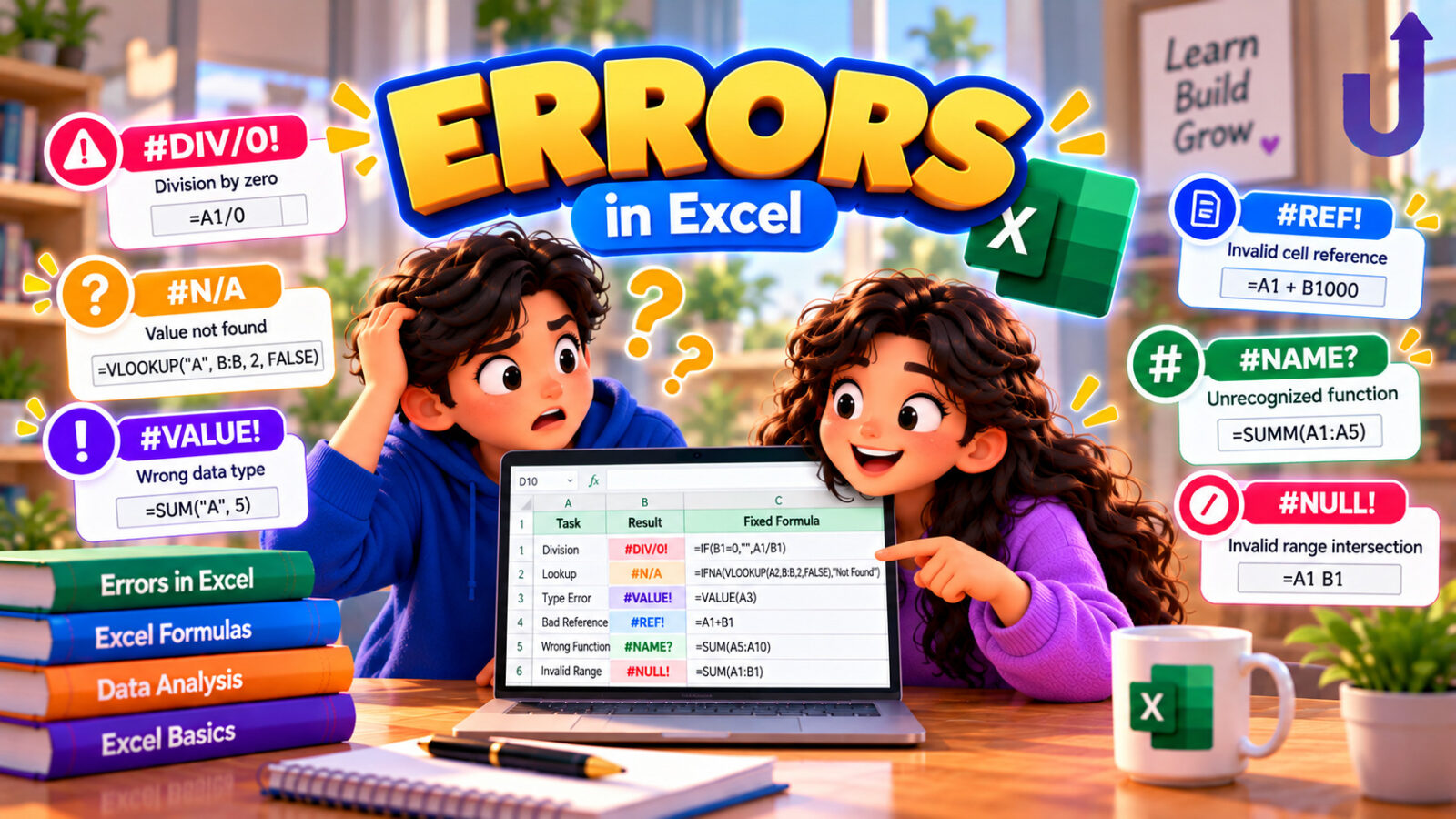
An Excel error value is a special result that starts with a hash sign, such as #N/A or #REF!, and tells you the formula could not produce a normal answer. Each error names a different problem: #DIV/0! is a division by zero, #N/A means a lookup found nothing, #VALUE! means a wrong type of value, #REF! means a cell reference is no longer valid, and so on. Formula auditing is the set of tools and habits for finding why a formula gives an error or a wrong number.
This guide lists every error with a formula that produces it, explains what usually causes each, shows how errors spread from cell to cell, when to hide them and when not to, and how to trace a problem through a workbook. Every result was produced by running the formula in Microsoft Excel.
In this guide
The short version
- Read the error name first: it points at the cause.
#N/Anot found,#VALUE!wrong type,#REF!deleted or invalid reference,#NAME?unknown name or typo,#DIV/0!divide by zero,#NUM!impossible number. - An error inside a range poisons
SUM.AGGREGATE(9, 6, range)skips errors. IFERRORhides every error, including your own mistakes. UseIFNAfor lookups.- Use Evaluate Formula and Trace Precedents to find where a wrong number starts.
Every error value at a glance
Each formula below produces exactly one error, typed into a small worksheet where A1:B3 hold the numbers 1 to 6:
| Formula | Excel shows | Why |
|---|---|---|
| =1/0 | #DIV/0! | #DIV/0!: division by zero |
| =NA() | #N/A | #N/A: value not available, the error a lookup gives when it finds nothing |
| =SUMM(1,2) | #NAME? | #NAME?: Excel does not recognise SUMM (a mistyped function name) |
| =SUM(A1:A2 B1:B2) | #NULL! | #NULL!: a space means intersection, and A1:A2 and B1:B2 share no cells |
| =SQRT(-1) | #NUM! | #NUM!: an impossible number, here the square root of a negative |
| =#REF!+1 | #REF! | #REF!: an invalid reference |
| ="a"+1 | #VALUE! | #VALUE!: text where a number is needed |
| =FILTER(A1:A3,A1:A3>100) | #CALC! | #CALC!: a dynamic array result with nothing in it |
Two more you may see. #SPILL! appears when a dynamic array formula is blocked by something in its way:
| A | |
|---|---|
| 1 | #SPILL! |
| 2 | x |
| 3 |
And a row of hash signs is not an error. It means the column is too narrow to show a number or date. Widen the column and the number is there:
| A | B | |
|---|---|---|
| 1 | ##### | #DIV/0! |
What causes each error
These formulas show typical situations. A1 holds 10, B1 holds 0, C1 is empty, D1 holds the text abc and E1 holds a text with just a space:
| Formula | Excel shows | Why |
|---|---|---|
| =A1/B1 | #DIV/0! | dividing by a zero |
| =A1/C1 | #DIV/0! | dividing by an empty cell counts as dividing by zero |
| =A1+D1 | #VALUE! | adding a number and the text abc |
| =A1+E1 | #VALUE! | a cell that looks empty but holds a space |
| =SUM(A1,D1) | 10 | SUM skips text in referenced cells, so no error |
| =A1&D1 | 10abc | joining with & never gives #VALUE!: the number becomes text |
| =VLOOKUP(10,A1:B1,3,FALSE) | #REF! | the key 10 is found, but column 3 does not exist in a two-column table: #REF! |
| =VLOOKUP(5,A1:B1,2,FALSE) | #N/A | the key 5 is not in the first column: #N/A |
| =IF(D1=abc,1,0) | #NAME? | abc without quotes is read as a name, which does not exist |
| =IF(D1="abc",1,0) | 1 | with quotes it is text, and the test works |
| =10^400 | #NUM! | the result is too big for Excel to hold |
| =LN(0) | #NUM! | the logarithm of zero is undefined |
| =A1+"" | #VALUE! |
#REF!: a reference that no longer exists
The classic cause is deleting a row, column or sheet that a formula points at. Here B1 held =A2*2 and row 2 was deleted:
Before: B1 holds =A2*2
| A | B | |
|---|---|---|
| 1 | 10 | 40 |
| 2 | 20 | |
| 3 | 30 |
What is inside the cells before the deletion
| A | B | |
|---|---|---|
| 1 | 10 | =A2*2 |
| 2 | 20 | |
| 3 | 30 |
After deleting row 2
| A | B | |
|---|---|---|
| 1 | 10 | #REF! |
| 2 | 30 |
B1 now points at nothing
| A | B | |
|---|---|---|
| 1 | 10 | =#REF!*2 |
| 2 | 30 |
Undo the deletion (Ctrl + Z) if you can. If you cannot, retype the reference. A VLOOKUP column number that is too big also gives #REF!, as the table above shows.
How errors spread
An error in one cell makes every formula that reads it an error too, and when two different errors meet, the first one Excel reads is the one you see. A1 holds 10, A2 holds =NA() and A3 holds =1/0:
| Formula | Excel shows | Why |
|---|---|---|
| =A2+A3 | #N/A | #N/A is read first |
| =A3+A2 | #DIV/0! | swap the order and #DIV/0! is read first |
| =SUM(A1:A3) | #N/A | one error in the range spoils the whole SUM (the first error in the range order) |
| =SUM(A3,A2) | #DIV/0! | the argument order decides again |
| =AGGREGATE(9,6,A1:A3) | 10 | function 9 is SUM, option 6 says ignore errors: only the 10 is added |
| =IFERROR(SUM(A1:A3),0) | 0 | IFERROR replaces the whole error with a value |
| =SUMIF(A1:A3,">5") | 10 | SUMIF only looks at cells that meet the criterion, and an error does not |
| =COUNT(A1:A3) | 1 | COUNT counts only real numbers |
| =COUNTA(A1:A3) | 3 | COUNTA counts errors as filled cells |
| =ISERROR(A2) | TRUE | any error |
| =ISNA(A2) | TRUE | only #N/A |
| =ISNA(A3) | FALSE | |
| =ISERR(A2) | FALSE | ISERR is TRUE for every error except #N/A |
| =ISERR(A3) | TRUE | |
| =ERROR.TYPE(A2) | 7 | ERROR.TYPE turns an error into a number: 7 is #N/A |
| =ERROR.TYPE(A3) | 2 | 2 is #DIV/0! |
| =ERROR.TYPE(A1) | #N/A | no error, so ERROR.TYPE itself returns #N/A |
| Error | ERROR.TYPE |
|---|---|
| #NULL! | 1 |
| #DIV/0! | 2 |
| #VALUE! | 3 |
| #REF! | 4 |
| #NAME? | 5 |
| #NUM! | 6 |
| #N/A | 7 |
Handling errors: IFERROR, IFNA and friends
IFERROR(value, if_error) replaces any error with the value you choose. That is exactly its danger: it also replaces the errors that tell you the formula is broken. IFNA replaces only #N/A, the error that means not found. The formula below has a bug: the column number 3 does not exist in the two-column table. Watch what each function does with it:
| Formula | Excel shows | Why |
|---|---|---|
| =IFERROR(VLOOKUP(101,A1:B2,3,FALSE),"not found") | not found | the bug is hidden: it looks like a legitimate not-found |
| =IFNA(VLOOKUP(101,A1:B2,3,FALSE),"not found") | #REF! | IFNA lets #REF! through, so you see the bug |
| =IFERROR(VLOOKUP(999,A1:B2,2,FALSE),"not found") | not found | a genuine miss: both show the message |
| =IFNA(VLOOKUP(999,A1:B2,2,FALSE),"not found") | not found | IFNA handles the normal case |
| =VLOOKUP(101,A1:B2,2,FALSE) | Asha | the correct formula |
The habit: use IFNA around lookups, use IF to guard a specific problem (for example IF(B1=0, "", A1/B1)), and keep IFERROR for cases where any failure really should show a fallback.
Blank cells versus empty text
A truly empty cell and a formula that returns empty text (="") look the same, but they behave differently in arithmetic. A1 is empty and A2 holds the formula ="":
| Formula | Excel shows | Why |
|---|---|---|
| =10/A1 | #DIV/0! | an empty cell counts as zero: #DIV/0! |
| =10/A2 | #VALUE! | empty text is text, not zero: #VALUE! |
| =A1+1 | 1 | an empty cell counts as zero in arithmetic |
| =A2+1 | #VALUE! | empty text cannot be added |
| =10/N(A2) | #DIV/0! | N() turns text into 0, so we get a division by zero |
| =SUM(A1:A2) | 0 | SUM skips text |
So a formula chain that returns "" in some rows can produce #VALUE! in the next column. Test with A2="" before you calculate, or use N().
Circular references
A circular reference is a formula that depends on its own result, directly or through other cells. Excel warns you, cannot calculate it, and shows 0 (unless iterative calculation is switched on, which you rarely want):
| A | |
|---|---|
| 1 | 0 |
| A | B | |
|---|---|---|
| 1 | 0 | 0 |
| A | |
|---|---|
| 1 | 1 |
| 2 | 2 |
| 3 | 3 |
| 4 | 4 |
| 5 | 0 |
The status bar shows the address of one cell in the loop, and Formulas, Error Checking, Circular References lists them. The usual fix is to change the range so it does not include the formula’s own cell, for example SUM(A1:A4).
Formula auditing tools
When a formula gives a wrong number, or an error you cannot explain, work backwards from the result. The tools are on the Formulas tab:
| Tool | What it does | Shortcut or place |
|---|---|---|
| Show Formulas | displays every formula instead of its result | Ctrl + ` (backtick) |
| Trace Precedents | draws arrows from the cells a formula reads | Formulas, Trace Precedents; Ctrl + [ selects them |
| Trace Dependents | draws arrows to the cells that read this cell | Formulas, Trace Dependents; Ctrl + ] selects them |
| Trace Error | follows an error back towards the cell that started it | Formulas, Error Checking, Trace Error |
| Evaluate Formula | steps through a formula one calculation at a time | Formulas, Evaluate Formula |
| F9 on a selection | replaces the selected part of a formula with its value, to see it (press Esc to undo) | in the formula bar |
| Error Checking | flags common problems with a green triangle | Formulas, Error Checking |
| Go To Special | selects all cells that hold formulas, errors, constants or blanks | F5, Special |
| Watch Window | keeps chosen cells visible while you work elsewhere | Formulas, Watch Window |
Two functions read a formula for you. FORMULATEXT shows another cell’s formula as text, and ISFORMULA tells you whether a cell holds one. A1 holds 5 and B1 holds =A1*2:
| Formula | Excel shows | Why |
|---|---|---|
| =FORMULATEXT(B1) | =A1*2 | the formula in B1 as text |
| =ISFORMULA(B1) | TRUE | |
| =ISFORMULA(A1) | FALSE | a constant |
| =ISFORMULA(C1) | FALSE | an empty cell |
A simple routine that solves most problems: select the cell, look at the formula bar, use Evaluate Formula to find the step where the value goes wrong, then check the inputs with Trace Precedents. Look for text that looks like numbers, hidden spaces and ranges of the wrong size before you suspect anything more exotic.
Common mistakes
Mistake 1: wrapping everything in IFERROR
It makes the sheet look clean and hides the bug. Keep errors visible while you build, and add handling for the specific case afterwards.
Mistake 2: ignoring #N/A because it looks harmless
A lookup that returns #N/A for a key that seems to be in the list usually means a text-versus-number mismatch or a hidden space, which affects real data.
Mistake 3: deleting rows without checking references
Before you delete a row, column or sheet, use Trace Dependents to see what reads it. A #REF! inside a formula is hard to repair after the fact.
Mistake 4: confusing a hash row with an error
A cell full of hash signs is a width problem. Double-click the column border to fit it.
Cheat sheet
| Error | Usual cause | First thing to check |
|---|---|---|
| #DIV/0! | divisor is zero or empty | IF(B1=0, "", A1/B1) |
| #N/A | lookup found nothing | text versus number, spaces, exact match |
| #VALUE! | wrong type, such as text in a calculation | cells with a space or text, empty text "" |
| #REF! | deleted or invalid reference | Ctrl + Z, or retype; column number in VLOOKUP |
| #NAME? | misspelled function or name, text without quotes | spelling, quotes, function available in your version |
| #NUM! | impossible number | SQRT of a negative, LN of zero, huge results |
| #NULL! | a space between two ranges | use a comma or a colon |
| #SPILL! | something blocks the result | clear the cells below and beside |
| #CALC! | an empty array result | the FILTER if_empty argument |
| ##### | column too narrow | double-click the column border |
Try it yourself
Work out each answer first, then open the solution.
1. A1 holds 10, A2 holds =NA() and A3 holds =1/0. What does =SUM(A1:A3) show, and which formula gives the total of the numbers only?
Show solution
=SUM(A1:A3) shows #N/A, the first error in the range. =AGGREGATE(9,6,A1:A3) shows 10, because option 6 ignores errors.
2. A1:B2 hold 101, Asha, 102 and Ravi. =VLOOKUP(101, A1:B2, 3, FALSE) shows an error. Which one, and why?
Show solution
It shows #REF!, because the table has only two columns and the formula asks for column 3. =IFNA(VLOOKUP(101,A1:B2,3,FALSE),"not found") lets that error through instead of hiding it, and the correct formula returns Asha.
3. D1 holds the text abc. =IF(D1=abc, 1, 0) shows #NAME?. Fix it.
Show solution
Put the text in quotes: =IF(D1="abc", 1, 0). Without quotes Excel reads abc as the name of something, and no such name exists. The corrected formula returns 1.
4. A1 holds =NA(). Which of ISERROR, ISNA and ISERR return TRUE?
Show solution
| Formula | Excel shows |
|---|---|
| =ISERROR(A1) | TRUE |
| =ISNA(A1) | TRUE |
| =ISERR(A1) | FALSE |
ISERR is TRUE for every error except #N/A, which makes it useful for finding real problems in a lookup column.
Frequently asked questions
What do the different error values mean in Excel?
#DIV/0! division by zero, #N/A value not available (a lookup found nothing), #NAME? unknown function or name, #NULL! ranges that do not intersect, #NUM! impossible number, #REF! invalid cell reference, #VALUE! wrong type of value, #SPILL! a blocked array result, and #CALC! an empty array.
How do I fix the #N/A error in Excel?
Find out why the lookup missed: a text-versus-number mismatch, a hidden space, a value that really is missing, or an approximate match on an unsorted list. If it is a real miss, handle it with IFNA or the not-found argument of XLOOKUP.
Why does Excel show #VALUE!?
A formula received the wrong kind of value, for example text in an addition. Check for cells with spaces or text, and for formulas that return empty text.
What causes #REF! in Excel?
A formula refers to a cell that no longer exists, usually because a row, column or sheet was deleted, or a VLOOKUP column number is larger than the table.
What is the difference between IFERROR and IFNA?
IFERROR replaces every error. IFNA replaces only #N/A, so other errors still show and reveal mistakes.
How do I sum a range that contains errors?
Use =AGGREGATE(9, 6, range) to ignore the errors, or fix the cells that produce them. SUM returns the first error in the range.
How do I find a circular reference?
Look at the address in the status bar, or use Formulas, Error Checking, Circular References. Then change the formula so it does not include its own cell.
How do I see what a formula is doing step by step?
Select the cell and use Formulas, Evaluate Formula. To test a part of a long formula, select it in the formula bar and press F9, then Esc to undo.
Test yourself
Timed questions on Errors and Formula Auditing, with an explanation for every answer.