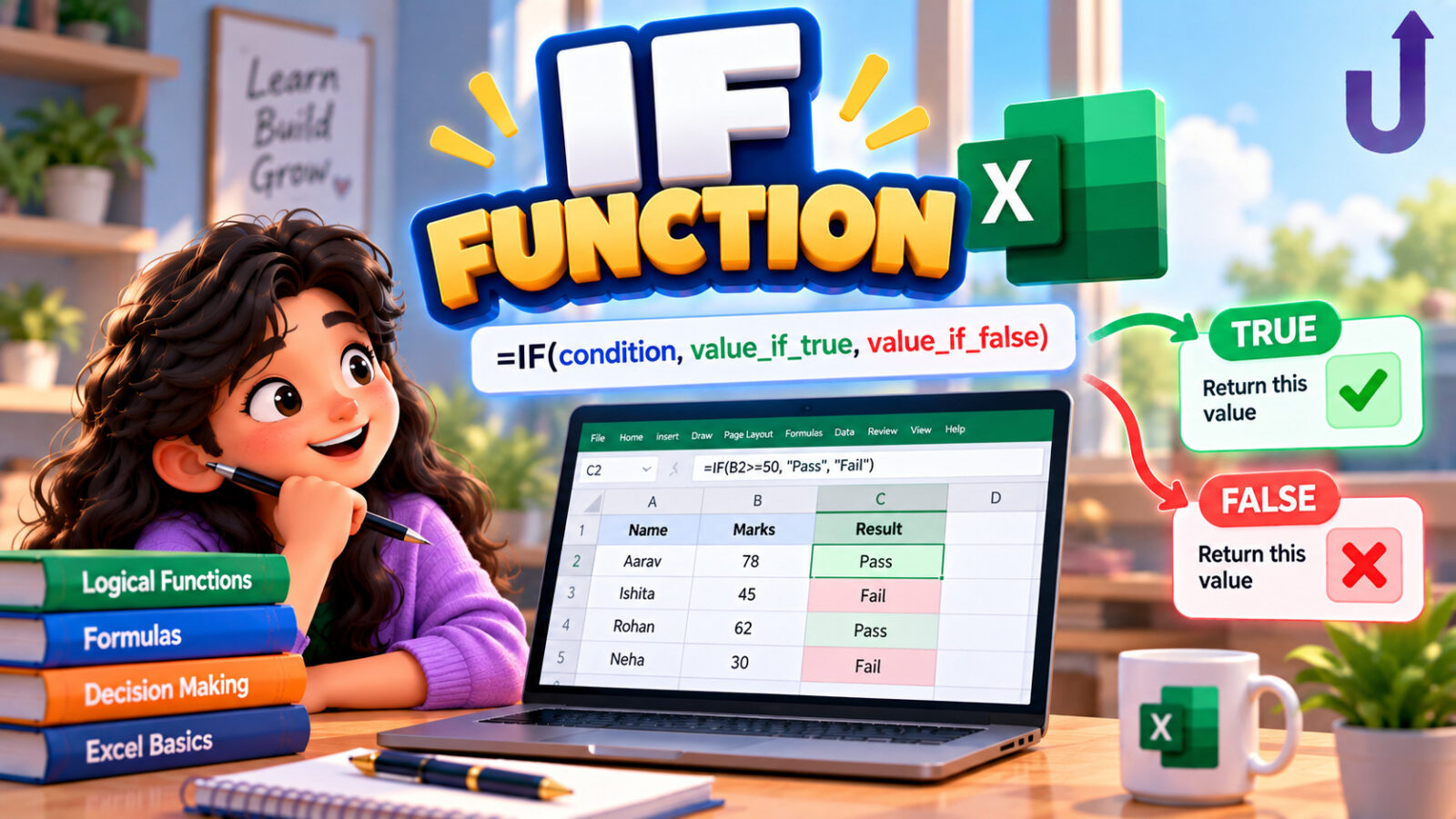
Logical functions in Excel test a condition and then either return TRUE or FALSE, or choose between results. The main ones are IF, AND, OR, NOT, IFS, SWITCH and the error handlers IFERROR and IFNA. IF is the one you will use most: =IF(condition, value_if_true, value_if_false) gives one answer when the condition is true and another when it is not.
This guide goes from a single comparison to nested IF, to combining AND with OR (where the placement of brackets changes the answer), and to the small details that make a correct-looking formula give a wrong result. Every result was produced by running the formula in Microsoft Excel.
In this guide
The short version
=IF(test, if_true, if_false). If you leave outif_falseand the test fails, Excel showsFALSE.- In a nested IF, Excel stops at the first true condition, so test the most specific one first.
ANDneeds every condition true,ORneeds at least one. Put anORinside anANDwith brackets, and check the brackets.IFSreplaces long nested IFs in Excel 2019 and 365, but needs a finalTRUEfor the default.
Comparisons and TRUE or FALSE
Every logical function starts from a comparison, which returns TRUE or FALSE. The operators are =, <> (not equal), >, <, >= and <=. A1 holds 15 and B1 holds the text Pune:
| Formula | Excel shows | Why |
|---|---|---|
| =A1>10 | TRUE | |
| =A1>=15 | TRUE | |
| =A1<>15 | FALSE | <> means not equal |
| =B1="pune" | TRUE | text comparison ignores upper or lower case |
| =B1="Pune " | FALSE | a trailing space makes it a different text |
| =(A1>10)*1 | 1 | TRUE counts as 1 in arithmetic |
| =TRUE+TRUE | 2 | and FALSE counts as 0 |
The IF function
IF takes a condition and two results. Text results go in double quotes. In column C every mark of 40 or more passes. Column D leaves out the value for a failed test:
What the sheet shows
| A | B | C | D | |
|---|---|---|---|---|
| 1 | Student | Marks | Result | No else |
| 2 | Asha | 82 | Pass | Pass |
| 3 | Ravi | 75 | Pass | Pass |
| 4 | Meera | 60 | Pass | Pass |
| 5 | John | 45 | Pass | Pass |
| 6 | Sam | 39 | Fail | FALSE |
What is inside the cells (Show Formulas)
| A | B | C | D | |
|---|---|---|---|---|
| 1 | Student | Marks | Result | No else |
| 2 | Asha | 82 | =IF(B2>=40,”Pass”,”Fail”) | =IF(B2>=40,”Pass”) |
| 3 | Ravi | 75 | =IF(B3>=40,”Pass”,”Fail”) | =IF(B3>=40,”Pass”) |
| 4 | Meera | 60 | =IF(B4>=40,”Pass”,”Fail”) | =IF(B4>=40,”Pass”) |
| 5 | John | 45 | =IF(B5>=40,”Pass”,”Fail”) | =IF(B5>=40,”Pass”) |
| 6 | Sam | 39 | =IF(B6>=40,”Pass”,”Fail”) | =IF(B6>=40,”Pass”) |
Look at D6: when the test fails and there is no value_if_false, Excel returns the word FALSE, which is rarely what you want in a report. Always give both results, even if the second is an empty text "".
Nested IF: several outcomes
When there are more than two outcomes, put another IF in the value_if_false place. Excel checks the conditions in order and stops at the first one that is true. That is why the order matters. Column C tests the highest band first; column D puts the lowest band first; column E uses > instead of >=:
| A | B | C | D | E | |
|---|---|---|---|---|---|
| 1 | Student | Marks | Right order | Wrong order | Uses > |
| 2 | Asha | 82 | A | C | A |
| 3 | Ravi | 75 | A | C | B |
| 4 | Meera | 60 | B | C | C |
| 5 | John | 45 | C | C | C |
| 6 | Sam | 39 | Fail | Fail | Fail |
| Column | Formula in row 2 | What is wrong or right |
|---|---|---|
| C Right order | =IF(B2>=75,"A",IF(B2>=60,"B",IF(B2>=40,"C","Fail"))) | the strictest condition comes first |
| D Wrong order | =IF(B2>=40,"C",IF(B2>=60,"B",IF(B2>=75,"A","Fail"))) | 82 is at least 40, so the first test wins: everyone who passes gets C |
| E Uses > | =IF(B2>75,"A",IF(B2>60,"B",IF(B2>40,"C","Fail"))) | exactly 75 is not greater than 75, so Ravi drops a grade |
Two rules come out of this. Order the tests from the strictest to the loosest (or the other way round with <), and decide whether a boundary value belongs to the upper or the lower band, then pick >= or > to match.
AND, OR and NOT
AND(cond1, cond2, ...) is TRUE only if all conditions are true. OR(...) is TRUE if at least one is true. NOT(cond) flips TRUE and FALSE. They usually sit inside an IF:
What the sheet shows
| A | B | C | D | E | F | |
|---|---|---|---|---|---|---|
| 1 | Student | Maths | Science | AND | OR | NOT(AND) |
| 2 | Asha | 82 | 71 | Pass | Pass | FALSE |
| 3 | Ravi | 35 | 90 | Fail | Pass | TRUE |
| 4 | Meera | 60 | 30 | Fail | Pass | TRUE |
| 5 | John | 20 | 25 | Fail | Fail | TRUE |
What is inside the cells
| A | B | C | D | E | F | |
|---|---|---|---|---|---|---|
| 1 | Student | Maths | Science | AND | OR | NOT(AND) |
| 2 | Asha | 82 | 71 | =IF(AND(B2>=40,C2>=40),”Pass”,”Fail”) | =IF(OR(B2>=40,C2>=40),”Pass”,”Fail”) | =NOT(AND(B2>=40,C2>=40)) |
| 3 | Ravi | 35 | 90 | =IF(AND(B3>=40,C3>=40),”Pass”,”Fail”) | =IF(OR(B3>=40,C3>=40),”Pass”,”Fail”) | =NOT(AND(B3>=40,C3>=40)) |
| 4 | Meera | 60 | 30 | =IF(AND(B4>=40,C4>=40),”Pass”,”Fail”) | =IF(OR(B4>=40,C4>=40),”Pass”,”Fail”) | =NOT(AND(B4>=40,C4>=40)) |
| 5 | John | 20 | 25 | =IF(AND(B5>=40,C5>=40),”Pass”,”Fail”) | =IF(OR(B5>=40,C5>=40),”Pass”,”Fail”) | =NOT(AND(B5>=40,C5>=40)) |
Ravi (35 in Maths, 90 in Science) fails the AND rule but passes the OR rule. John fails both.
AND with an OR inside: where the brackets go
Real rules combine both: “call the lead if the city is Pune and either the order is at least 500 or the person is a member”. Condition A must always hold, and condition B is one of two alternatives, so the OR goes inside the AND:
=IF(AND(B2="Pune", OR(C2>=500, D2="Yes")), "Call", "Skip")
Move the brackets and the rule changes. Column F below is OR(AND(city is Pune, order at least 500), member), which means “Pune with a big order, or any member”. It looks almost the same and gives different answers for John and Zoya, who are members outside Pune:
| A | B | C | D | E | F | |
|---|---|---|---|---|---|---|
| 1 | Name | City | Order | Member | A: AND(city, OR(..)) | B: OR(AND(..), member) |
| 2 | Asha | Pune | 700 | No | Call | Call |
| 3 | Ravi | Pune | 300 | Yes | Call | Call |
| 4 | Meera | Mumbai | 900 | No | Skip | Skip |
| 5 | John | Mumbai | 200 | Yes | Skip | Call |
| 6 | Sam | Pune | 100 | No | Skip | Skip |
| 7 | Zoya | Delhi | 800 | Yes | Skip | Call |
The rule for the brackets: whatever is inside OR( ) is one alternative choice for a single slot of the AND. Say the rule out loud in words first, then place the brackets to match the words. The same logic appears in other tools: in FILTER it is (city="Pune")*((order>=500)+(member="Yes")), where * means AND and + means OR.
IFS and SWITCH
IFS(test1, result1, test2, result2, ...) checks the tests in order and returns the result of the first true one. It avoids the nested brackets. It exists in Excel 2019 and Microsoft 365, not in Excel 2016 or earlier. If nothing matches, IFS returns #N/A, so end with TRUE as a catch-all:
| A | B | C | D | |
|---|---|---|---|---|
| 1 | Student | Marks | IFS with TRUE at the end | IFS without a default |
| 2 | Asha | 82 | A | A |
| 3 | Ravi | 75 | A | A |
| 4 | Meera | 60 | B | B |
| 5 | John | 45 | C | C |
| 6 | Sam | 39 | Fail | #N/A |
SWITCH(value, match1, result1, match2, result2, ..., default) compares one value with a list of exact matches, which suits codes and labels:
| Formula | Excel shows | Why |
|---|---|---|
| =SWITCH(A1,1,"Mon",2,"Tue",3,"Wed","Other") | Tue | 2 matches the second pair |
| =SWITCH(A2,1,"Mon",2,"Tue",3,"Wed","Other") | Other | nothing matches, so the default is used |
| =SWITCH(A2,1,"Mon",2,"Tue",3,"Wed") | #N/A | no default given: #N/A |
IFERROR and IFNA
IFERROR(value, if_error) replaces any error with a value you choose. IFNA(value, if_na) replaces only #N/A, the error that lookups give when nothing is found. Prefer IFNA when you expect only that case, because IFERROR also hides real mistakes such as a wrong range:
| Formula | Excel shows | Why |
|---|---|---|
| =A1/B1 | #DIV/0! | division by zero |
| =IFERROR(A1/B1,"check the divisor") | check the divisor | IFERROR catches it |
| =IFNA(A1/B1,"x") | #DIV/0! | IFNA lets #DIV/0! through |
| =IFNA(NA(),"not found") | not found | IFNA catches #N/A |
What Excel evaluates and what it skips
IF only evaluates the branch it picks, so it can guard against an error in the other branch. AND and OR evaluate every argument, so an error in a later argument spoils the answer even if an earlier one already decided it. A1 holds 0:
| Formula | Excel shows | Why |
|---|---|---|
| =IF(A1=0,"skipped",10/A1) | skipped | the division is never evaluated |
| =IF(TRUE,"ok",1/0) | ok | the error branch is skipped |
| =OR(A1=0,10/A1>1) | #DIV/0! | OR still evaluates 10/A1 and fails |
| =IF(A1=0,TRUE,10/A1>1) | TRUE | the safe version: IF decides first |
| =AND(FALSE,1/0) | #DIV/0! | AND does not short-circuit either |
Gotchas with comparisons
A1 holds 15, A2 holds the text 100, A3 holds the number 100 and A4 is empty:
| Formula | Excel shows | Why |
|---|---|---|
| =10<=A1<=20 | FALSE | does not test a range: (10<=15) is TRUE, and TRUE<=20 is FALSE |
| =AND(A1>=10,A1<=20) | TRUE | the correct way to test a range |
| =A2=A3 | FALSE | text 100 and number 100 are different |
| =A2=VALUE(A2) | FALSE | so the text does not equal its converted self |
| ="abc">100 | TRUE | text is always greater than any number |
| =A4=0 | TRUE | an empty cell equals 0 … |
| =A4="" | TRUE | … and equals empty text |
| =IF(0,"yes","no") | no | zero counts as FALSE |
| =IF(5,"yes","no") | yes | any other number counts as TRUE |
When nested IF gets too long
Excel allows up to 64 levels of nesting, but nobody should read that. If the bands are a list, put them in a table and let a lookup pick the band. Here the four bands are written as an array constant inside VLOOKUP with approximate matching (the last argument TRUE), which finds the largest lower limit that does not exceed the mark. In a real workbook you would put the band table in cells and point at it:
What the sheet shows
| A | B | C | |
|---|---|---|---|
| 1 | Student | Marks | Grade from a table |
| 2 | Asha | 82 | A |
| 3 | Ravi | 75 | A |
| 4 | Meera | 60 | B |
| 5 | John | 45 | C |
| 6 | Sam | 39 | Fail |
What is inside the cells (Show Formulas)
| A | B | C | |
|---|---|---|---|
| 1 | Student | Marks | Grade from a table |
| 2 | Asha | 82 | =VLOOKUP(B2,{0,”Fail”;40,”C”;60,”B”;75,”A”},2,TRUE) |
| 3 | Ravi | 75 | =VLOOKUP(B3,{0,”Fail”;40,”C”;60,”B”;75,”A”},2,TRUE) |
| 4 | Meera | 60 | =VLOOKUP(B4,{0,”Fail”;40,”C”;60,”B”;75,”A”},2,TRUE) |
| 5 | John | 45 | =VLOOKUP(B5,{0,”Fail”;40,”C”;60,”B”;75,”A”},2,TRUE) |
| 6 | Sam | 39 | =VLOOKUP(B6,{0,”Fail”;40,”C”;60,”B”;75,”A”},2,TRUE) |
The lookup functions are covered in detail in the lookup guide of this series.
Cheat sheet
| Goal | Formula | Note |
|---|---|---|
| Two outcomes | =IF(B2>=40,"Pass","Fail") | always give both results |
| Several outcomes | =IF(B2>=75,"A",IF(B2>=60,"B","C")) | strictest test first |
| All conditions | =AND(A1>=18, A1<=60) | test a range with two comparisons |
| Any condition | =OR(B1="Yes", C1>=500) | |
| A and (B or C) | =AND(A1, OR(B1, C1)) | the OR sits inside the AND |
| (A and B) or C | =OR(AND(A1, B1), C1) | a different rule from the one above |
| Many bands, Excel 2019+ | =IFS(B2>=75,"A",B2>=40,"C",TRUE,"Fail") | TRUE as the default |
| Match a code | =SWITCH(A1,1,"Mon",2,"Tue","Other") | exact matches only |
| Hide an error | =IFERROR(A1/B1,"") | IFNA if only #N/A is expected |
Try it yourself
Work out each answer first, then open the solution.
1. Commission is 10% for sales of 10,000 or more, 5% for 5,000 or more, and 2% otherwise. Write one formula for the first row and check it on 12,000, 5,000 and 4,999.
Show solution
What the sheet shows
| A | B | C | |
|---|---|---|---|
| 1 | Rep | Sales | Commission rate |
| 2 | Asha | 12000 | 10% |
| 3 | Ravi | 5000 | 5% |
| 4 | Meera | 4999 | 2% |
What is inside the cells (Show Formulas)
| A | B | C | |
|---|---|---|---|
| 1 | Rep | Sales | Commission rate |
| 2 | Asha | 12000 | =IF(B2>=10000,0.1,IF(B2>=5000,0.05,0.02)) |
| 3 | Ravi | 5000 | =IF(B3>=10000,0.1,IF(B3>=5000,0.05,0.02)) |
| 4 | Meera | 4999 | =IF(B4>=10000,0.1,IF(B4>=5000,0.05,0.02)) |
Test the highest band first. 5,000 gets 5% because the test is >=, and 4,999 drops to 2%.
2. Write a test that is TRUE only when A1 is between 18 and 60 inclusive, and check it on 18, 60, 61 and 17.
Show solution
| Formula | Excel shows |
|---|---|
| =AND(A1>=18,A1<=60) | TRUE |
| =AND(A2>=18,A2<=60) | TRUE |
| =AND(A3>=18,A3<=60) | FALSE |
| =AND(A4>=18,A4<=60) | FALSE |
Use AND with two comparisons. The shortcut 18<=A1<=60 does not work in Excel.
3. A1 holds 35. What does =IF(A1>=40,"Pass") return?
Show solution
| Formula | Excel shows |
|---|---|
| =IF(A1>=40,"Pass") | FALSE |
With no value_if_false, IF returns FALSE, not an empty cell.
4. What do =OR(TRUE,1/0) and =IF(TRUE,1,1/0) return?
Show solution
| Formula | Excel shows |
|---|---|
| =OR(TRUE,1/0) | #DIV/0! |
| =IF(TRUE,1,1/0) | 1 |
OR evaluates all its arguments, so the division fails. IF only evaluates the branch it chooses.
Frequently asked questions
What is the IF function in Excel?
IF(logical_test, value_if_true, value_if_false) tests a condition and returns one result if it is TRUE and another if it is FALSE.
How do I use IF with AND and OR in Excel?
Put AND(...) or OR(...) as the first argument: =IF(AND(B2>=40, C2>=40), "Pass", "Fail"). To combine them, nest one inside the other, for example AND(A1, OR(B1, C1)).
How many IF statements can you nest in Excel?
Up to 64 levels in modern versions of Excel, but readable formulas rarely go beyond three or four. Use IFS, SWITCH or a lookup table instead.
What is the difference between IF and IFS?
IF handles two outcomes and needs nesting for more. IFS takes pairs of test and result and returns the first true one, without nesting. IFS is available in Excel 2019 and Microsoft 365.
Why does my IF formula return FALSE?
Usually because the test failed and the formula has no value for that case: =IF(A1>=40,"Pass"). Add a third argument.
Why does IF give the wrong grade in a nested formula?
Excel stops at the first condition that is true. If the loosest condition comes first, everyone matches it. Test the strictest condition first.
What is the difference between IFERROR and IFNA?
IFERROR catches every error type. IFNA catches only #N/A, so it does not hide mistakes such as #DIV/0! or #REF!.
Is text comparison in Excel case sensitive?
No. ="pune"="PUNE" is TRUE. Use EXACT(a, b) when you need a case-sensitive comparison.
Test yourself
Timed questions on Logical Functions, with an explanation for every answer.